Arjun did great in Class 8. He knows AI learns from data. He's used ChatGPT, tried Python in Colab, and even built a simple sorting algorithm. But one question still bothers him: "When I feed data into a neural network, what is actually happening inside?"
His teacher says "the network adjusts its weights." But what does that really mean? Today we'll open the black box together — and by the end, Arjun (and you) will be able to draw a diagram of a neural network and explain exactly what happens at each step.
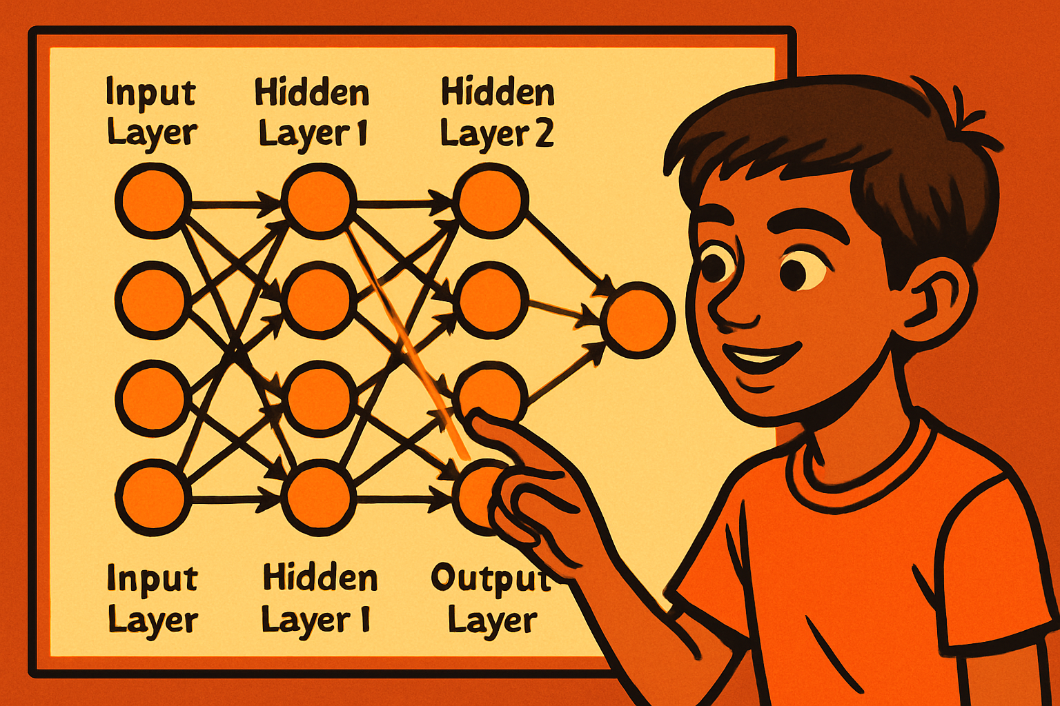
From Class 8, we know that a neural network is inspired by the human brain. It takes input, processes it through layers, and produces an output (a prediction). But we treated the inside as a "black box." Now we open it.
Every neural network is made of layers stacked one after another. There are exactly three types:
H = Hours studied · A = Attendance % · S = Sleep hours → P = Pass/Fail probability
Every connection between two nodes has a number called a weight. The weight says: "how much should this input influence the next node?" A large positive weight means "pay a lot of attention." A weight near zero means "almost ignore this."
A DJ's mixing board has sliders (volume for each instrument). The neural network's weights are those sliders. Training adjusts the sliders until the output sounds right. Before training, the sliders are set randomly. After training, they're at the exact positions that produce correct predictions.
In a tiny network with 3 inputs and 4 hidden nodes, there are already 3 × 4 = 12 weights just for the first layer. Large modern networks have billions of weights — GPT-4 has roughly 1.7 trillion parameters.
Each node in a hidden or output layer does two simple things:
Multiply each input by its weight, add them all together, then add one more number called the bias. Result: z = (w₁×x₁) + (w₂×x₂) + ... + bias
Pass the sum z through an activation function. This decides whether this node "fires" and with what intensity. Common functions: ReLU, Sigmoid, Softmax.
When you give a trained network an input, data flows forward through the layers, one layer at a time. Each layer produces a set of numbers that become the input to the next layer. This one-way trip is called the forward pass.
# Tiny neural network forward pass (concept — no framework)
import math

# Input: [hours_studied=6, attendance=0.85, sleep=7]
x = [6, 0.85, 7]

# Weights for 2 hidden nodes (made-up values for illustration)
w = [[0.4, 0.1, 0.3],   # weights for hidden node 1
     [0.2, 0.5, 0.1]]   # weights for hidden node 2
bias = [0.2, 0.1]

# Step 1: Weighted sum
z1 = sum(w[0][i]*x[i] for i in range(3)) + bias[0]
z2 = sum(w[1][i]*x[i] for i in range(3)) + bias[1]

# Step 2: ReLU activation
def relu(z): return max(0, z)
h1, h2 = relu(z1), relu(z2)

print(f"Hidden node 1 output: {h1:.4f}")
print(f"Hidden node 2 output: {h2:.4f}")
# These then feed forward to the output layer...
Run this in Google Colab and try changing the weights to see how the output changes. This is exactly what training does automatically — but using calculus.
Training a neural network means finding the right weights. The algorithm that does this is called backpropagation. Here's the intuition:
Feed an input through the network to get a predicted output.
Compare prediction to the correct answer. The "loss" is a number that tells how wrong we are. Lower loss = better model.
Using calculus (the chain rule), calculate how much each weight contributed to the error. This is the "gradient."
Adjust each weight by a tiny amount in the direction that reduces the loss. The size of the step is called the learning rate.
Each repetition through the full training dataset is called an epoch. After many epochs, the weights stabilise and the loss is low.
Imagine you're blindfolded on a hilly landscape. Your goal: find the lowest valley. You feel the slope under your feet (the gradient) and take one small step downhill. Then check the slope again, take another step. Repeat until you can't go any lower. That valley is the lowest loss — the best set of weights.
A shallow network (1–2 hidden layers) can learn simple patterns — like whether a student passes based on study hours. A deep network (many hidden layers) can learn complex patterns — like recognising a face in a photo, translating a language, or generating realistic text.
Each layer learns to detect increasingly complex features:
- Layer 1: Detects simple patterns (edges in images, common words in text)
- Layer 2: Combines those into shapes (curves, phrases)
- Layer 3+: Combines those into objects (faces, sentences, meanings)
Here's a minimal neural network you can run right now in Google Colab. It trains on made-up student data to predict exam pass/fail:
# Open Colab: colab.research.google.com → New Notebook

import numpy as np
from tensorflow import keras

# Fake student data: [hours_studied, attendance, sleep_hours]
X = np.array([[2, 0.5, 5], [7, 0.9, 8], [4, 0.7, 6],
              [1, 0.3, 4], [8, 0.95, 8], [3, 0.6, 6]])
y = np.array([0, 1, 1, 0, 1, 0])  # 0=fail, 1=pass

# Build a simple neural network
model = keras.Sequential([
    keras.layers.Dense(4, activation='relu', input_shape=(3,)),
    keras.layers.Dense(1, activation='sigmoid')
])

model.compile(optimizer='adam', loss='binary_crossentropy',
              metrics=['accuracy'])

history = model.fit(X, y, epochs=100, verbose=0)
print(f"Final accuracy: {history.history['accuracy'][-1]:.2f}")

# Predict for a new student: [5 hours, 80% attendance, 7 hours sleep]
prediction = model.predict([[5, 0.8, 7]])
print(f"Pass probability: {prediction[0][0]:.2f}")