Image Classification with Transfer Learning 🖼️

# Transfer Learning with MobileNetV2 — Google Colab
# Example: Flower classifier (or replace with any image dataset)

import tensorflow as tf
from tensorflow import keras
from tensorflow.keras import layers
from tensorflow.keras.applications import MobileNetV2
import matplotlib.pyplot as plt
import numpy as np

# ── Step 1: Load dataset ──
# Using tf_flowers dataset as a stand-in for your own photos
# For your own images, use ImageDataGenerator.flow_from_directory()
import tensorflow_datasets as tfds

(ds_train, ds_val, ds_test), info = tfds.load(
    'tf_flowers',
    split=['train[:70%]', 'train[70%:85%]', 'train[85%:]'],
    as_supervised=True,
    with_info=True
)
NUM_CLASSES = info.features['label'].num_classes  # 5 flower types
print(f"Classes: {info.features['label'].names}")

# ── Step 2: Preprocess (resize and normalise) ──
IMG_SIZE = 224  # MobileNetV2 expects 224×224

def preprocess(image, label):
    image = tf.image.resize(image, [IMG_SIZE, IMG_SIZE])
    image = tf.cast(image, tf.float32) / 255.0
    return image, label

BATCH_SIZE = 32
ds_train = ds_train.map(preprocess).shuffle(1000).batch(BATCH_SIZE).prefetch(1)
ds_val   = ds_val.map(preprocess).batch(BATCH_SIZE).prefetch(1)
ds_test  = ds_test.map(preprocess).batch(BATCH_SIZE).prefetch(1)

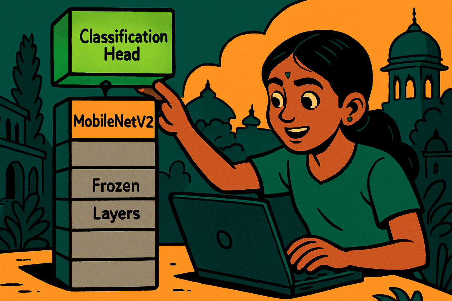
# ── Step 3: Load MobileNetV2 base (frozen) ──
base_model = MobileNetV2(
    input_shape=(IMG_SIZE, IMG_SIZE, 3),
    include_top=False,    # remove ImageNet classification head
    weights='imagenet'    # download pre-trained weights
)
base_model.trainable = False  # FREEZE — don't retrain these layers
print(f"Base model parameters: {base_model.count_params():,}")

# ── Step 4: Add classification head ──
inputs  = keras.Input(shape=(IMG_SIZE, IMG_SIZE, 3))
x       = base_model(inputs, training=False)  # frozen base
x       = layers.GlobalAveragePooling2D()(x)  # pool feature maps → 1D vector
x       = layers.Dense(128, activation='relu')(x)
x       = layers.Dropout(0.3)(x)
outputs = layers.Dense(NUM_CLASSES, activation='softmax')(x)

model = keras.Model(inputs, outputs)
model.compile(
    optimizer='adam',
    loss='sparse_categorical_crossentropy',
    metrics=['accuracy']
)
print(f"Trainable parameters: {sum([tf.size(w).numpy() for w in model.trainable_variables]):,}")

# ── Step 5: Phase 1 — Train the head only ──
print("\nPhase 1: Training classification head...")
history1 = model.fit(ds_train, epochs=5, validation_data=ds_val)

# ── Step 6: Phase 2 — Fine-tune top layers of base model ──
# Unfreeze the top 30 layers for fine-tuning
base_model.trainable = True
for layer in base_model.layers[:-30]:
    layer.trainable = False

# Recompile with a lower learning rate (important!)
model.compile(
    optimizer=keras.optimizers.Adam(learning_rate=1e-5),
    loss='sparse_categorical_crossentropy',
    metrics=['accuracy']
)

print("\nPhase 2: Fine-tuning top layers...")
history2 = model.fit(ds_train, epochs=10, validation_data=ds_val)

# ── Step 7: Evaluate on test set ──
test_loss, test_acc = model.evaluate(ds_test)
print(f"\nTest accuracy after fine-tuning: {test_acc:.2%}")

# ── Step 8: Predict on a single image ──
flower_names = info.features['label'].names
for images, labels in ds_test.take(1):
    preds = model.predict(images[:5])
    for i in range(5):
        print(f"Predicted: {flower_names[np.argmax(preds[i])]:15s}  "
              f"Actual: {flower_names[labels[i].numpy()]}")

# If you have your own images, organise them like this:
#
# my_dataset/
# ├── train/
# │   ├── healthy/       (put healthy fruit photos here)
# │   ├── diseased/      (put diseased fruit photos here)
# │   └── unripe/
# ├── val/
# │   ├── healthy/
# │   ├── diseased/
# │   └── unripe/
# └── test/
#     ├── healthy/
#     ├── diseased/
#     └── unripe/

from tensorflow.keras.preprocessing.image import ImageDataGenerator

# Augment training images to improve generalisation
train_datagen = ImageDataGenerator(
    rescale=1./255,
    rotation_range=20,
    horizontal_flip=True,
    zoom_range=0.2,
    shear_range=0.1
)
val_datagen = ImageDataGenerator(rescale=1./255)

train_gen = train_datagen.flow_from_directory(
    'my_dataset/train',
    target_size=(224, 224),
    batch_size=32,
    class_mode='sparse'
)
val_gen = val_datagen.flow_from_directory(
    'my_dataset/val',
    target_size=(224, 224),
    batch_size=32,
    class_mode='sparse'
)

# Replace ds_train / ds_val with train_gen / val_gen in model.fit()
# Google Colab: upload zip of your dataset with files.upload() or mount Google Drive